Regression: R functions for multiple regression and its ramifications
Note: Given the limited time availability in the workshop, we will cover only a subset of the following material in the Workshop. However, Chapters 11 and 12 of MFin 604 will rely heavily on some of the material shown below.
(a) Data modelling - Basics
In this section we will look at sales/advertising/income data and consider simple and multiple linear regression models.
a.1 Sales vs. advertising
 vs.
vs. 
Example: Let's use the sales and advertising data and analyze it.
-
Here is the graph of this data set as obtained by Rcmdr.
-
How did Rcmdr find the green line on the graph? This is the regression line, and here is what we do to find it. (To find the regression equation, you will need to use Rcmdr's Statistics > Fit Models > Linear Regression.) So, the regression line is Sales = 51.489 + 7.527 x Advertising with R-squared = 0.24. What do these numbers mean?
-
It is very important to look at the Pr(> | t |) values to get a feel for how significant is a coefficient. You can consider the ratio of Estimate to Std. Error (which gives the t value) as a Signal-to-Noise ratio. If this ratio is high [and the Pr(.) is low] then the coefficient is non-zero and so the result is significant. The values indicated by *, **, etc., indicate the significance codes (smaller code, the more significant is the coefficient.)
>>Predictions
How do we predict the sales for given advertising levels and also find prediction and confidence intervals?
- The next two commands are used to do the predictions:
- newPoint <- data.frame(ADVT=10.25); newPoint
- predict(RegModel.1,newPoint,interval="prediction")
- With the help of Rcmdr, we get these results. (The highlighted commands are entered manually in the Rcmdr window. The package UsingR and its function simple.lm is optional.) Note that with a single R line we can easily obtain the prediction results.
- Good news! Basically, the only time you will need to enter commands in Rcmdr is when you are doing predictions. We will do this one more time with multiple regression below. We will also look at a nice correlation plot (corrplot) package where you will enter a few simple commands. All other commands are generated by Rcmdr automatically.
Here are a few more examples of predictions. The inputs and results should be clear from the context.
newPoints <- data.frame(ADVT=c(8:11))
newPoints
ADVT
1 8
2 9
3 10
4 11
predict(RegModel.1,newPoints,interval="prediction")
fit
lwr upr
1 112.0672 79.10412 145.0304
2 119.5945 88.28846
150.9005
3 127.1217 96.49693 157.7466
4 134.6490 103.66509 165.6329
You could also enter
newPoints <- data.frame(ADVT=c(8,9.2,10.7))
to predict for 8, 9.2 and 10.7.
This is also possible:
newPoints <- data.frame(ADVT=c(seq(8,10.5,by=0.5)))
if you want to predict for 8, 8.5, 9, 9.5, 10, 10.5
-
R documentation for linear model lm().
-
Background material on linear regression from Wikipedia.
Exercise: Consider this house price dataset for 124 houses. Do a simple regression with Price as dependent variable and SqrFt as independent variable. Perform analysis similar to what we did above with the advertising/sales problem. (Answer: Regression equation is Price = 259.88 + 120.16 x SqrFt.)
a.2 Sales vs. advertising and income
-
R documentation for linear model lm().
 vs.
vs.  and
and 
Example: Now we use the sales vs. advertising and income data. So, this is a multiple regression problem which is solved as follows:
-
Rcmdr can plot the 3D graph of the dataset and even show the fitted linear surface. It also finds the coefficients of the regression equation. The results are here without the 3D graph. (To find the regression equation, you will need to use Rcmdr's Statistics > Fit Models > Linear Regression.) The regression equation is then Sales = 36.894 + 5.069 x Advertising + 0.808 x Income with R-squared = 0.45.
-
The comments made about the significance of the coefficients also apply here.
-
We should be able to predict the Sales from the given values of Advertising and Income. This is quite easy with R and the results are found here. (Note again that the highlighted commands are entered manually in the Rcmdr window.) The confint() command used here gives the 95% confidence intervals for the regression coefficients.
-
Background material on linear regression from Wikipedia.
Exercise: Consider the same house price dataset for 124 houses used above. Now use SqrFt, LotSize, Bedrooms and Bathrooms as independent variables and Price as dependent variable and perform a multiple regression.
Example : Here's an amazing example of four problems with very diffrent datasets which give the same results. Anscombe's quartet.
QUESTION: How long does it take R to run a multiple regression with 1,000,000 observations on 100 variables? Can MegaStat do it?
a.3 House Prices
-
R documentation for linear model lm().

Example: This is a more challenging problem with qualitative factors (such as Yes/No, North/West/East) for some variables in the dataset. To find the regression equation, you will need to use Rcmdr's Statistics > Fit Models > Linear Model as LinearModel.1 <- lm(Price ~ Bathrooms + Bedrooms + Brick + Neighborhood + Offers + SqFt, data=Dataset). The confint(LinearModel.1) command will produce the confidence intervals for coefficients. Here are the results.
(b) Data modelling - Making models more flexible
Dummy variables are needed when some of the variables assume binary values. Including interaction terms aid the analyst to obtain more accurate results in regression.
b.1 "Dummy" variables
-
R documentation for linear model lm().

Example: Let's consider the dataset for salaries. When we ignore the gender and plot the dataset, we are missing out on the information inherent in the gender differences. Only when we plot the data according to gender group, we see a more clear picture. The Rcmdr results are here. So, if we just consider the Experience and Salary columns, the regression equation is found as Salary = 59033.1 + 1727.3 x Experience. But is this accurate?
*****
Example: Here, we need to use a dummy variable to distinguish between males and females. We define Gender.Male = 1 if gender is "male" and 0 otherwise. The new dataset with this information is here. Using RegModel.3 <- lm(Salary~Experience+Gender.Male, data=Dataset), we find Salary = 53260.0 + 1744 x Experience + 17020 x Gender.Male. (R-squared = 0.31.)
Note: Of course, there is an easier way to do this with Rcmdr without using the Gender.Male construct. Just use the "Linear model". Rcmdr knows that Gender is a factor. If you pick it as an independent variable, R figures out the rest and you get the same result as Salary = 53260 + 1744 x Experience + 17020 x Gender[T.Male].
-
Starting salary for females is 53,260.
-
Starting salary for males is 53,260 + 17,020 = 70,280. (Discrimination?)
-
Each additional year of experience is worth 1,744 for either gender. (Seems strange! We will fix this soon with an interaction term.)
-
The Rcmdr results of this analysis.
Exercise: Use this dataset to estimate the travel time given, (i) distance travelled, (ii) number of deliveries and (iii) truck type. Note that truck type is a factor here and Rcmdr recognizes it. (Answer: 0.5222 + 0.0464 x Km + 0.7102 x Deliveries + 0.9 x TruckType[T.Van].)
b.2 Interaction terms
-
R documentation for linear model lm().

Example: We noted above that each additional year of experience is 1,744 for either gender. But this is not quite logical. Could it be more for males? We analyse this using an interaction term in the form Gender.Exp.Int = Gender.Male x Experience. The dataset with the interaction term is here. The regression equation is obtained as Salary = 66,333 + 666 x Experience - 8,034 x Gender.Male + 2,086 x Gender.Exp.Int. (R-squared = 0.55.)
Now what happens?
-
For females, Gender.Males = 0, so Salary = 66,333 + 666 x Experience. (Meaning?)
-
For males, it is more complicated: Since Gender.Males = 1, Salary = 66,333 + 666 x Experience - 8,034 x 1 + 2,086 x 1 x Experience. Simplifying we have Salary = 58,299 + 2,752 x Experience. (Meaning?)
Note 1: Of course, as before, there is an easier way to do this with Rcmdr without using the Gender.Exp.Int construct. Just use the "Linear model" and incorporate the product of Gender and Exp as a new variable. Rcmdr figures out what to do and finds exactly the same result. You can do this as an Exercise.
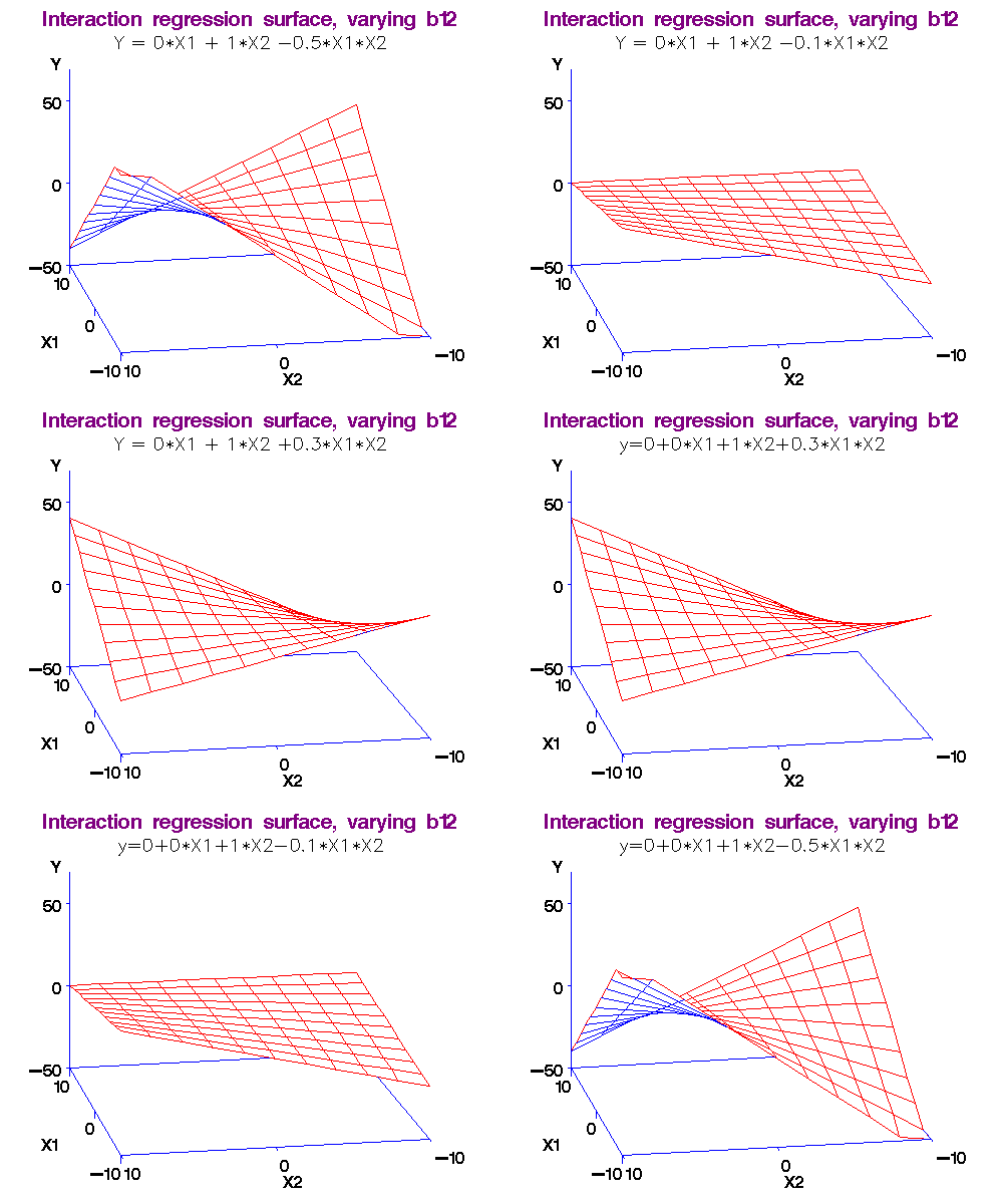
Note 2: What exactly do we mean by "interaction." I will make this more clear in the workshop by comparing two functions: (i) f(x,y) = ax + by, and (ii) f(x,y) = ax + by + cxy. In the first case, there is no interaction between x and y, but in the second there is! (Just find the partial derivative of f(x,y) w.r.t. variable y in both cases and you will see the difference.)
(c) Data modelling - Making models more selective
c.1 Multicollinearity
-
R documentation for linear model lm().

Is it always a good idea to include as many independent variables as we can in a regression problem? No! Let's see why.
Example: Consider the dataset for a problem with sales and assets as independent variables and profit as the dependent variable.
-
If we include both sales and assets in our problem we find very high p-values for both (0.340 and 0.643) indicating that they are not individually significant, and so they are useless! However, the F-value for the model is very small (0.002), now indicating that the model with these two variables the model is significant. There is also a high R-squared value (0.63). How could this be?
-
There is more to this. When we run the regression with a single variable (Profit vs. Sales, and Profit vs. Assets) we get logical results. Individually, both variables are significant! So, all of this tells us that jointly the two variables do not contribute to our understanding, but individually, they do.
-
The reason is that these variables are highly correlated as we see in the correlation matrix.
-
Here are the results from Rcmdr.
-
How do we cure this problem? By "Variable Selection."
Exercise: Use this dataset to find a regression equation for Time as dependent variable and Km, Deliveries and Gas (consumed) as independent variables. Is there a high correlation between Km and Gas? What can go wrong with such problems?
c.2 Variable selection by stepwise regression
-
R documentation for stepwise regression.
R has a nice way of dealing with the multicollinearity problem using stepwise regression.
Example: We use the same dataset as above. The stepwise procedure is applied after the regression problem is solved by using Models > Stepwise Model Selection... Here is the result.
-
We use the Akaike Information Criterion (AIC) and the backward/forward direction.
-
Smaller the AIC, the better is the model.
-
Start: AIC = 175.64 and Profit ~ Assets + Sales
-
If we remove Assets, we get the smallest AIC value 173.92.
-
Any further removal (of Sales) results in a higher AIC, so we stop.
-
Thus, we have Profit = -124.85492 + 0.02918 x Sales.
Exercise: Consider again the house price dataset for 124 houses. Run a regression with Price as the dependent variable and everything else (except SubDiv) as independent variable. Next, use Models > Stepwise Model Selection... and reduce the model with Akaike Information Criterion (AIC) and the backward/forward direction. How many independent variables do you have left and what is the AIC? (Answer: We have 5 variables left as Price ~ Bathrooms + Bedrooms + Distance + LotSize + SqrFt, and AIC is 736.41.)